A.M.C. Davies
Norwich Near Infrared Consultancy, 75 Intwood Road, Cringleford, Norwich NR4 6AA, UK. [email protected]
Introduction
You may realise that it is over two years since I began this series of “Back to Basics” (B2B). It has become something of an embarrassment because I keep finding gaps in what I have written. As we will see later; gaps are important! Before the start of the B2B series I wrote a column about “Separating the wheat from the chaff”,1 which was concerned with the latest method of spectral pre-treatment—orthogonal signal correction (OSC). In passing, I mentioned most of the pre-treatments in use today without any comment. In the latest column2 on PLS, I mentioned pre-treatments without any introduction and finished by saying that next time we would see if any other pre-treatments would give us improved results. That will have to wait; this column is about the most basic of pre-treatments, which has been used in spectroscopy well before the word “Chemometrics” was invented.
Derivatives
Derivative spectroscopy came into use in the “old days” when spectra were recorded by analogue recorders drawing a continuous black line on a white piece of paper (I wonder how many readers actually remember using them!). Derivatives are mathematically defined as the slope of the line at any given point and analogue recorders were available to do this in real time so that they could plot the derivative spectrum. If we take the derivative of a derivative (usually called a second derivative) this gives the slope of the first derivative so it is in fact the rate of change of slope of the original spectrum, you can continue with third and fourth derivatives or more but I would be surprised if you find them useful.
Nowadays spectra are recorded digitally so the rest of this column is about “pseudo” derivatives rather than true derivatives because the basic idea is that we can get something that behaves like the derivative by subtracting adjacent points along the original spectrum. Thus the derivative at λn is given by xn – xn – 1 where x is the measured spectrum at λn. First derivatives remove an additive baseline shift so this is very useful in NIR spectroscopy. However, first derivatives produce peaks where the original spectrum had maximum slope and crosses zero where the original had a peak and are thus rather difficult to interpret. NIR spectra also tend to have linear baseline increases and these are removed by second derivatives which have negative peaks where the original had a peak and are thus more readily comprehensible. For these reasons second derivatives are often preferred. A second derivative is the derivative of a first derivative so the formula, xn – 1 – 2xn + xn + 1 can be deduced. Figure 1 shows a peak and its first and second derivative. I have changed the scales so that they all plot in the same area. Now you can see that there is a problem. The second derivative, especially, looks noisy. Taking derivatives decreases the scale and increases the noise. There are two simple ways of improving this performance, averaging over segments and leaving gaps between the points used for the computation. Both are used. (Note that the computation moves across the spectrum like a window and all points will be used and computed except that we will lose a few points at the ends of the spectrum).

Segments and gaps
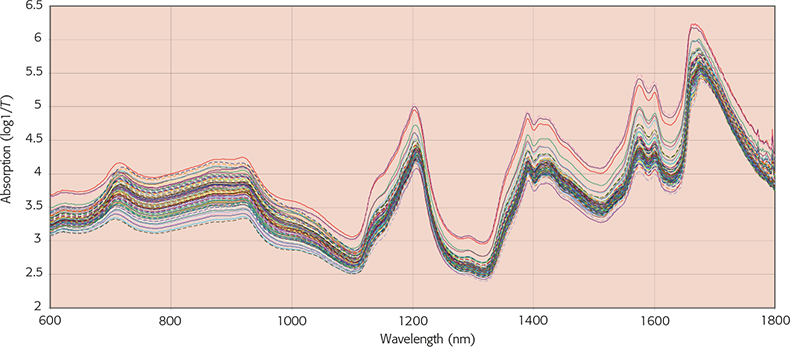
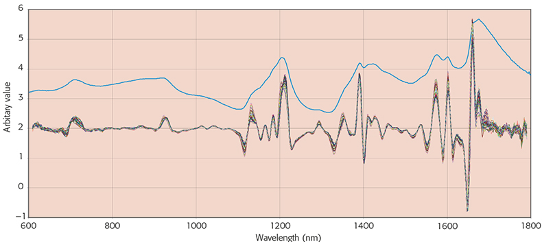
In Figure 2, I have plotted the second derivative spectrum of the spectrum in Figure 1 with increasing segment sizes and you will see that in addition to reducing the noise the apparent number of peaks also reduces. In Figure 3 I have plotted the same peak using an increasing gap and then combined the two approaches. Karl Norris has been very interested in gaps because his software can optimise the gap for each absorption that is used by his multiple regression program. He has shown3 that the gap should be similar in width to the absorption being utilised. However, Karl’s software is not commercially available so this very detailed optimisation of derivatives is not generally needed. The effect of an unvaried computation on the first hundred spectra in the “Shootout” data2 can be seen in Figures 4 and 5. Figure 4 shows the original spectra while Figure 5 shows the first original spectrum and then the second derivative of the first hundred using a gap of three and a segment of five. In this computation I also multiplied by –1 so that the peaks become positive and it is easy to see how they correspond to the original.

Figure 4. The first hundred original spectra from the “Shootout” data.2

Figure 5. The first, original spectrum (blue line), and the second derivative spectra of the first hundred spectra from the “Shootout” data.2 Derivatives were computed using a gap of three and a segment of five.
Savitzky–Golay
I will mention that derivatives can also be computed by the method of Savitsky and Golay.4 It is quite complex, so if you would like a full explanation you need to consult a book.5 In brief, the method fits a curve through a small section of the spectrum and then finds the slope of the tangent to this curve at the central point. This is the first derivative at that point. As we have seen earlier, the second derivative can be computed from the first and in a similar way Savitsky–Golay derivatives reduce to a series of linear combinations of the measured absorbances so they may be difficult to understand but the computations are trivial for your friendly PC! These are applied as a moving window across the whole spectrum. You do have choices in the number of points in the window and the order of the polynomial (but my suggestion is to stop with quadratics).
Convolution functions for the segment/gap method
David Hopkins6 has shown that the segment/gap method can also be reduced to the application of a moving set of weights. So the whole of this article could be replaced by a few tables of weights but I want you to understand the principle!
Conclusions
Derivatives are very useful functions for removing some of the extraneous signals from NIR spectra. However, (unless you have Karl Norris’s software and knowledge) the resulting spectra still contain multiplicative effects of light scattering and the performance of methods such as PLS will be improved if these can be reduced. In my next column we will look at two popular methods for achieving it.
References
- A.M.C. Davies and T. Fearn, “Sorting the wheat from the chaff”, Spectroscopy Europe 14(2), 16 (2002). https://www.spectroscopyeurope.com/td-column/sorting-wheat-chaff
- A.M.C. Davies, “Back to basics: running your first PLS calibration”, Spectroscopy Europe 18(6), 28 (2006). https://www.spectroscopyeurope.com/td-column/back-basics-running-your-first-pls-calibration
- K.H. Norris, “Understanding and correcting the factors which affect diffuse transmittance spectra”, NIR news 12(3), 6 (2001). doi: https://doi.org/10.1255/nirn.613
- A. Savitzky and M.J.E. Golay, “Smoothing and differentiation of data by simplified least squares procedures”, Anal. Chem. 36, 1627 (1964). doi: https://doi.org/10.1021/ac60214a047
- T. Næs, T. Isaksson, T. Fearn and T. Davies, A User-Friendly Guide to Multivariate Calibration and Classification. NIR Publications, Chichester (2002). l
- D.W. Hopkins, “What is a Norris derivative?”, NIR news 12(3), 3 (2001). doi: https://doi.org/10.1255/nirn.611


