Matthew Cassap
>Senior Applications Specialist, Thermo Fisher Scientific, Cambridge, UK. E-mail: [email protected]
Introduction
The presence of trace elements in gasoline can lead to a number of detrimental effects both on the automobile engine using the fuel as well as the environment. Trace elements can dramatically decrease engine performance by negatively impacting the operation of the engine’s electronic sensors that control the combustion process. Additionally, environmental pollution occurs when trace elements are transported from the engine to the environment via emissions. The analysis of these elements is therefore crucial to ensure that the performance of the engine is not affected by the fuel and that environmental damage does not occur when trace elements are released from the engine via emissions. This article discusses how modern inductively-coupled plasma (ICP) technology surpasses the performance of traditionally used atomic absorption spectroscopy (AAS) techniques to ensure optimal fuel quality.
A common example of a trace element present in gasoline is lead, which not only affects the performance of an engine by poisoning the catalytic converter, but is also transported into the environment via exhaust emissions. Once in the environment, lead can enter the food chain via different pathways such as soils, water, plants and bio-accumulate, causing adverse effects or even death due to its high toxicity. Silicon is another trace element that can cause severe degradation of engine performance. This was demonstrated when a fuel depot in Southern England supplied a large proportion of the UK’s automobile filling stations with gasoline contaminated with silicon. This caused the oxygen sensor within some engines to fail causing automobiles to misfire and experience a dramatic loss of power. Two possible sources of the contamination were identified. According to the first hypothesis, an octane-enhancing agent was blended with the fuel. The second theory claimed that the fuel was stored or transported in a tank that had previously stored diesel containing an anti-foaming agent based on a silicon compound, which had not been washed or emptied properly.
A dependable analytical method is therefore necessary to provide accurate monitoring of trace elements in gasoline in order to ensure finest fuel quality and enable best engine performance and protection of the environment.
Traditional techniques for gasoline analysis
Atomic absorption spectroscopy (AAS) has traditionally been used to monitor the concentrations of trace elements in gasoline. However, this is a single-element analysis technique, with which sample preparation and subsequent analysis can be rather challenging. Plasma-based methods, such as inductively coupled plasma-optical emission spectrometry (ICP-OES) and inductively coupled plasma-mass spectrometry (ICP-MS), have emerged as ideal alternatives offering multi-elemental capabilities.
ICP-MS offers lower detection limits than ICP-OES, but it can suffer from a number of limitations when analysing organic matrices, including carbon deposition on the interface, interferences from carbon-based molecules and sample introduction challenges. ICP-OES is a more robust technique, requiring much less method development. Nevertheless, two key challenges must be overcome to effectively analyse gasoline with ICP-OES. The first is the high volatility of gasoline. When a volatile liquid is introduced into an ICP-OES instrument via the nebuliser, a large amount of vapour is produced. The vapour makes the plasma unstable and causes it to be extinguished. The second challenge is that different gasoline blends have different volatilities depending on the climate they are blended for. For example, in warmer climates gasoline is less volatile, which reduces vaporisation in the fuel lines of an engine. This can cause vapour-lock, preventing the fuel pump from working correctly. As a consequence, when samples with different volatiles are aspirated, different amounts are transported to the plasma and false concentrations of the trace elements are reported.
Overcoming the challenges
Gasoline volatility can be lowered by reducing the fuel’s temperature. As a result, the amount of fuel that will be vaporised by the nebuliser will be decreased and the fuel will be directly introduced into the plasma. To achieve this, the spray chamber must be cooled to approximately –40°C.
An alternative method to decrease gasoline volatility is to use a miscible solvent with a lower vapour pressure, such as kerosene, to dilute the fuel. A large dilution factor of approximately 20 is required to reduce the vapour pressure sufficiently for room temperature analysis. Unfortunately, such large dilution factors degrade the method detection limits significantly.
A third method involves using a nebuliser with a flow rate of 75 µL min–1 or less. By introducing a small amount of solvent into the plasma per unit time, the vapour pressure exerted on the plasma from the fuel is minimal and the plasma stability is not affected. Nevertheless, this method reduces sensitivity slightly and due to the low flow rate, the analysis time is increased.
For ease of use, one approach is to use a combination of a cooled spray chamber and dilution of the fuel with a less volatile solvent. If gasoline is diluted with a lower volatility solvent, it will evaporate at a much slower rate making it easier to handle. This dilution also means that the temperature of the spray chamber can be increased from –40°C to around –15°C. The spray chamber will therefore reach a stable temperature in a shorter period of time. This higher temperature is easier to achieve with typical off-the-shelf Peltier-cooled spray chambers.
Different volatilities of different gasoline blends can be overcome using an internal standard. The use of an internal standard can also correct for any loss of volume of the gasoline sample due to evaporation of highly volatile organic compounds, which is likely to occur at a low rate during sample analysis.
Experimental
The Thermo Scientific iCAP 6500 ICP-OES radial view was used for this analysis due to its ability to optimise the radial viewing height in order to minimise interferences from matrix elements such as carbon. A Glass Expansion IsoMist temperature-controlled spray chamber was implemented to reduce the temperature of the spray chamber to –15°C for the purposes of the experiment. The temperature controlled spray chamber was used in conjunction with a glass concentric nebuliser.
Standards were prepared by diluting a Conostan S21, 300 mg kg–1, oil-based standard in petroleum ether with 40–60°C boiling range. 15 g of kerosene containing 1 mg kg–1 of yttrium (diluted from Conostan 5000 mg kg–1 oil-based yttrium standard) was then added to the solution, giving a total mass of 30 g. Yttrium was used as an internal standard for the analysis to correct for differences in volatility between standards and samples and losses due to evaporation. Calibration standards were prepared at the concentrations shown in Table 1.
| Standard | Concentration |
| Blank | 0 mg kg–1 |
| Calibration standard 1 | 0.07 mg kg–1 |
| Calibration standard 2 | 0.257 mg kg–1 |
| Calibration standard 3 | 0.649 mg kg–1 |
| Calibration standard 4 | 1.184 mg kg–1 |
Gasoline samples were prepared by weighing the sample and then adding the same mass of kerosene containing 1 mg kg–1 yttrium. Spikes of the sample were also prepared in the same manner as the standards but using the gasoline sample instead of the petroleum ether for the initial dilution.
Method development
The temperature-controlled spray chamber was set to a temperature of –15°C. A solution of 1 : 1 petroleum ether (40–60°C) and kerosene was aspirated into the plasma. The nebuliser and auxiliary gas flows were adjusted until the base of the plasma was half-way between the top of the auxiliary tube and the bottom of the load coil and the sample channel was just below the top of the outer tube. The plasma parameters and sample introduction configuration used for the analysis are shown in Table 2.
| Parameters | Setting |
| RF power | 1600 W |
| Nebuliser gas flow | 0.2 L min–1 |
| Auxiliary gas flow | 1 L min–1 |
| Coolant gas flow | 14 L min–1 |
| Radial viewing height | 12 mm |
| Pump speed | 50 rpm |
| Pump tubing (drain only) | White/white solvent flex |
| Nebuliser | Glass concentric |
| Spray chamber | IsoMist |
| Spray chamber temperature | –15°C |
| Centre tube | 1 mm |
| Torch | Enhanced matrix tolerance |
The sub-array plots (see, for example, Figure 1) for each of the wavelengths were examined to ensure freedom from interference. When a peak at a neighbouring wavelength was identified, using the wavelength finder function of the instrument software (Thermo Scientific iTEVA Software), the affected background point was moved to ensure that false negative results were not obtained. Figure 1 shows that a titanium wavelength had a neighbouring peak from a chromium wavelength that may interfere with the background subtraction measurement. If the background correction point was located on the chromium peak, too much background would be taken away from the titanium (sample analyte peak) and the result obtained would be significantly lower than it should be. By simply moving the background point in the sub-array display, this issue was easily resolved.
 which could cause a possible interference on the background correction point. Moving the left background correction point to a new position (highlighted at ca 334.92 nm) avoids this problem.")
The instrument was then calibrated with the prepared calibration standards and the samples and spikes were analysed. A detection and quantification limit study was carried out by analysing a ten replicate blank solution prepared in the same manner as the calibration blank. The standard deviation of these ten replicates was then multiplied by three (3-sigma) and by the dilution factor (two) to ascertain the detection limit (DL). For the quantification limit study, the standard deviation was multiplied by ten and then by the dilution factor. These studies were repeated three times and the average detection and quantification limits were determined using the mean of the values obtained. A two-hour stability study continuously analysed spiked sample to demonstrate the long-term precision of the method.
Results and discussion
Table 3 demonstrates the results of the sample, spike recovery, detection and quantitation limit studies. These results show that spike recoveries for all elements determined were well within acceptable limits of ±10% of the prepared value of 0.87 mg kg–1, with the exception of boron for which the recovery was somewhat high. This is likely to be due to the instability of boron in this matrix and the addition of a commercially available stabiliser may solve this problem. The method detection limits were also acceptable with most of them being in the low µg kg–1 range.
| Sample (mg kg–1) | Spike (mg kg–1) | Recovery (%) | Method direction limit (mg kg–1) | Method quantification limit (mg kg–1) | |
| Ag 338.389 nm | 0.04 | 0.89 | 102 | 0.017 | 0.056 |
| Al 308.215 nm | <DL | 0.94 | 107 | 0.095 | 0.316 |
| B 208.595 nm | 0.08 | 1.11 | 127 | 0.061 | 0.203 |
| Ba 223.527 nm | 0.01 | 0.87 | 100 | 0.007 | 0.024 |
| Ca 184.00 nm | 0.75 | 0.93 | 107 | 0.041 | 0.137 |
| Cd 214.438 nm | 0.01 | 0.82 | 94 | 0.003 | 0.009 |
| Cr 267.716 nm | 0.01 | 0.86 | 99 | 0.010 | 0.035 |
| Cu 324.754 nm | 0.02 | 0.87 | 100 | 0.009 | 0.031 |
| Fe 238.204 nm | <DL | 0.89 | 102 | 0.017 | 0.057 |
| Mg 279.553 nm | 0.07 | 0.89 | 101 | 0.001 | 0.002 |
| Mn 293.930 nm | 0.01 | 0.87 | 100 | 0.009 | 0.032 |
| Mo 281.615 nm | <DL | 0.89 | 102 | 0.022 | 0.074 |
| Ni 231.604 nm | <DL | 0.87 | 100 | 0.028 | 0.094 |
| P 178.284 nm | 0.52 | 0.94 | 108 | 0.061 | 0.205 |
| Pb 220.353 | <DL | 0.86 | 98 | 0.038 | 0.127 |
| Si 212.412 nm | <DL | 0.88 | 100 | 0.032 | 0.108 |
| Sn 289.999 nm | <DL | 0.86 | 99 | 0.110 | 0.366 |
| Ti 334.941 nm | 0.01 | 0.85 | 98 | 0.004 | 0.012 |
| V 309.311 nm | 0.01 | 0.90 | 103 | 0.005 | 0.016 |
| Zn 213.856 nm | 0.56 | 1.01 | 105 | 0.003 | 0.009 |
The results of the stability run are presented graphically in Figure 2. These were also within acceptable limits. The first sample of this study was within 10% of the prepared value of 0.4105 mg kg–1 and for the duration of the study deviation from within these limits was not seen.
.")
Conclusion
Trace elements in gasoline severely degrade engine performance and pollute the environment in the form of exhaust gases. It is therefore essential that the concentrations of trace elements in gasoline are regularly monitored to eliminate these negative effects. ICP-OES is a powerful method capable of analysing trace elements in gasoline with a simple dilution of the sample with a lower volatility solvent and a temperature controlled spray chamber set to –15°C. The use of an internal standard corrects for any differential transport effects caused by volatility variation and for the differential concentration effects arising from evaporation. Overall, the technique offers low detection limits, good long-term stability and unmatched precision.